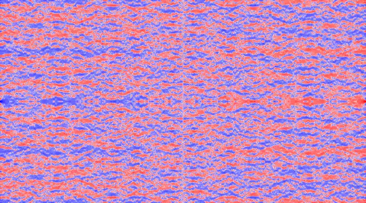
Air Hockey Phase Space
After a night out at a barcade a few years back, I came home and began to think about the phase space of an air hockey game. To be precise, given a position on the table \((x_0, y_0)\) and a velocity vector with direction specified by an angle \(\theta\), will the puck go into my goal, my opponent’s goal, or just bounce between walls forever? For simplicity, I’m assuming a perfectly frictionless table surface and perfectly elastic collisions. A diagram of the idealized air hockey table, with a coordinate system and relevant variables and parameters, is shown to the right. These parameters are:
-
\(s_x\) : length of table in \(x\) dimension, taken to be 1.0 in non-dimensionalized length units
-
\(s_y\) : length of table in \(y\) dimension, taken to be 1.8 in non-dimensionalized length units
-
\(w\) : width of goal, taken to be 0.16 in non-dimensionalized length units,
with values of these parameters taken from these websites.
The strategy employed for finding the final destination of the puck consists of calculating the intersection point of the puck with a particular wall and changing the angle consistent with the law of reflection, repeating the process until the puck lands within the goal, or the maximum number of bounces is reached. The intersection point can be calculated explicitly using basic algebra: based on the definition of \(\theta\), the slope at which the puck will travel is \(-\frac{1}{\tan \theta}\). By rearranging the expression for point-slope form, we get the equations
[\begin{aligned}
y &= \frac{1}{\tan \theta} (x_0 - x) + y_0
x &= \tan \theta (y_0 - y) + x_0,
\end{aligned}]
which can be solved for the intercepts at \(x=0\), \(x=s_y\), \(y=0\), or \(y=s_y\), depending on the value of \(\theta\). The algorithm for the function nextPoint, which computes the location of the next intersection point of the puck with the border of the table, as well as the rebound angle, is displayed below:

The animation to the left shows the paths a puck takes for a series of angles, when its initial location is the center of the table. Small changes in \(\theta\) can result in significant changes to the end state of the puck, as evidenced by the rapidly changing lines. This sensitive dependence on initial conditions is a hallmark of chaotic systems and suggests that the behavior or the air hockey table system is more complicated than its simple geometry suggests. In practical terms, that means that we can probably use this system to generate some cool looking plots!
In order to study the phase space of the air hockey table in a more systematic way, we define a new function, bounceScore, which quantifies how “good” a single shot is for a given initial location and shot angle, that is based on the number of bounces the puck engages in before entering into one of the two goals. To distinguish between the two goals and maintain continuity, we define the function such that a value of -1 indicates the puck went into your goal before the first bounce, a value of 1 indicates the puck went into your opponent’s goal before the first bounce, and a value of 0 indicates the puck did not end up in either goal after a set number of bounces.
An algorithm to compute the bounceScore function is shown below. I originally implemented it in Python, but that was too slow for my liking, so I later switched to Fortran. A lot of people seem to think Fortran is a dead language, but I like using it for high-performance applications because of its native support for array operations, ease of parallelization using OpenMP/MPI, and interfaceability with Python through f2py.
Implementing these algorithms requires addressing a few numerical issues related to avoiding the asymptotic behavior of \(\tan \theta\) and and \(\frac{1}{\tan \theta}\) at \(\theta = \pm \frac{\pi}{2}\) and \(\theta = \pi\) respectively, but I’m neglecting that here in order to keep the algorithms simple. You can look at my code on GitHub if you’re curious.
The goal width \(w\) is an important parameter for the system. On one extreme with \(w=0\), all shot angles for all locations never make it into a goal, so bounceScore is always zero. On the other extreme with \(w=s_x\), any \(\theta_0\) between \(-\frac{\pi}{2}\) and \(+\frac{\pi}{2}\) yields a positive bounceScore and any \(\theta_0\) between \(\frac{\pi}{2}\) and \(\frac{3 \pi}{2}\) yields a negative bounceScore. Both of these extremes are boring, but the values of \(w\) between 0 and \(s_x\) produce interesting results.
The video below shows the bounceScore at all locations, averaged over all angles, as \(w\) loops between 0 and \(s_x\), i.e. each pixel represents a particular location on the table. I rotated the table by 90 degrees because it fit better on the page that way. The color indicates which of the two goals the puck is likeliest to end up in, with blue indicating your goal, and red indicating your opponent’s goal. For visualization purposes, I raised the bounceScore to the power of 0.25 to increase the contrast, but that doesn’t affect the underlying pattern of blue and red regions.

The phase space of the air hockey table is 5 dimensional (\(x_0, y_0, \theta_0, \frac{w}{s_x}, \frac{s_y}{s_x}\)), so visualizing its entirety on a 2D computer screen is impossible. The best we can do is visualizing selected 2D or 3D slices and animating an additional dimension. The above video can be thought of as a sum over the \(\theta\) dimension and an animation over the \(\frac{w}{s_x}\) dimension, with \(\frac{s_y}{s_x}\) held constant.
The video below shows three different views of a phase space slice with the \(\frac{w}{s_x}\) and \(\frac{s_y}{s_x}\) dimensions held constant, with animations over the \(x\), \(y\), and \(\theta\) dimensions respectively.

